Design of Experiments May Be Used With Discerete

Design of experiments (DOE) is used to understand the effects of the factors and interactions that impact the output of a process. As a battery of tests, a DOE is designed to methodically build understanding and enhance the predictability of a process. A DOE investigates a list of potential factors whose variation might impact the process output. These factors can be derived from a variety of sources including process maps, FMEAs, Multi-Vari studies, Fishbone Diagrams, brainstorming techniques, and Cause and Effect Matrices. With most data-analysis methods, you observe what happens in a process without intervening. With a designed experiment, you change the process settings to see the effect this has on the process output. The term design of experiments refers to the structured way you change these settings so that you can study the effects of changing multiple settings simultaneously. This active approach allows you to effectively and efficiently explore the relationship between multiple process variables (x's) and the output, or process performance variables (y's). This tool is most commonly used in the Analyze step of the DMAIC method as an aid in identifying and quantifying the key drivers of variation, and in the Improve step as an aid in selecting the most effective solutions from a long list of possibilities.

Introduction

• DOE identifies the "vital few" sources of variation (x's)—the factors that have the biggest impact on the results
•  DOE identifies the x's that have little effect on the results
• It quantifies the effects of the important x's, including their interactions
• It produces an equation that quantifies the relationship between the x's and the y's
• It predicts how much gain or loss will result from changes in process conditions

The types of DOEs include:

• Screening DOEs, which ignore most of the higher order interaction effects so that the team can reduce the candidate factors down to the most important ones.
• Characterization DOEs, which evaluate main factors and interactions to provide a prediction equation. These equations can range from 2^k designs up to general linear models with multiple factors at multiple levels. Some software packages readily evaluate nonlinear effects using center points and also allow for the use of blocking in 2^k analyses.
•  Optimizing DOEs, which use more complex designs such as Response Surface Methodology or iterative simple designs such as evolutionary operation or plant experimentation to determine
  the optimum set of factors.
• Confirming DOEs, where experiments are done to ensure that the prediction equation matches reality.

Classical experiments focus on 1FAT (one factor at a time) at two or three levels and attempt to hold everything else constant (which is impossible to do in a complicated process). When DOE is properly constructed, it can focus on a wide range of key input factors or variables and will determine the optimum levels of each of the factors. It should be recognized that the Pareto principle applies to the world of experimentation. That is, 20% of the potential input factors generally make 80% of the impact on the result.
The classical approach to experimentation, changing just one factor at a time, has shortcomings:

• Too many experiments are necessary to study the effects of all the input factors.
• The optimum combination of all the variables may never be revealed.
•  The interaction (the behavior of one factor may be dependent on the level of another factor) between factors cannot be determined.
• Unless carefully planned and the results studied statistically, conclusions may be wrong or misleading.
• Even if the answers are not actually wrong, non-statistical experiments are often inconclusive. Many of the observed effects tend to be mysterious or unexplainable.
• Time and effort may be wasted by studying the wrong variables or obtaining too much or too little data.

The design of experiments overcomes these problems by careful planning. In short, DOE is a methodology of varying a number of input factors simultaneously, in a carefully planned manner, such that their individual and combined effects on the output can be identified. Getting good results from a DOE involves a number of steps:

• Set objectives
• Select process variables
• Select an experimental design
• Execute the design
• Check that the data are consistent with the experimental assumptions
• Analyze and interpret the results
• Use/present the results (may lead to further runs or DOES)

Applications of DOE

Situations, where experimental design can be effectively used include:

• Choosing between alternatives
• Selecting the key factors affecting a response
• Response surface modeling to:
  • Hit a target
  • Reduce variability
  • Maximize or minimize a response
  • Make a process robust (despite uncontrollable "noise" factors)
  • Seek multiple goals

Advantages of DOE:

• Many factors can be evaluated simultaneously, making the DOE process economical and less interruptive to normal operations.
•  Sometimes factors having an important influence on the output cannot be controlled (noise factors), but other input factors can be controlled to make the output insensitive to noise factors.
• ln-depth, statistical knowledge is not always necessary to get a big benefit from standard planned experimentation.
•  One can look at a process with relatively few experiments. The important factors can be distinguished from the less important ones. Concentrated effort can then be directed at the important ones.
• Since the designs are balanced, there is confidence in the conclusions drawn. The factors can usually be set at the optimum levels for verification.
• If important factors are overlooked in an experiment, the results will indicate that they were overlooked.
• Precise statistical analysis can be run using standard computer programs.
• Frequently, results can be improved without additional costs (other than the ( costs associated with the trials). In many cases, tremendous cost savings can be achieved.

DOE Terms

Understanding DOEs requires an explanation of certain concepts and terms.

1. Alias: An alias occurs when two-factor effects are confused or confounded with each other. Alias occurs when the analysis of a factor or interaction cannot be unambiguously determined because the factor or interaction settings are identical to another factor or interaction, or is a linear combination of other factors or interactions. As a result, one might not know which factor or interaction is responsible for the change in the output value. Note that aliasing/confounding can be additive, where two or more insignificant effects add and give a false impression of statistical validity. Aliasing can also offset two important effects and essentially cancel them out.
2. Balanced: A fractional factorial design, in which an equal number of trials design (at every level state) is conducted for each factor. A balanced design will have an equal number of runs at each combination of the high and low settings for each factor.
3. Block: A subdivision of the experiment into relatively homogeneous experimental units. The term is from agriculture, where a single field would be divided into blocks for different treatments.
4. Blocking: When structuring fractional factorial experimental test trials, blocking is used to account for variables that the experimenter wishes to avoid. A block may be a dummy factor that doesn't interact with the real factors. Blocking allows the team to study the effects of noise factors and remove any potential effects resulting from a known noise factor. For example, an experimental design may require a set of eight runs to be complete, but there is only enough raw material in a lot to perform four runs. There is a concern that different results may be obtained with the different lots of material. To prevent these differences, should they exist, from influencing the results of the experiment, the runs are divided into two halves with each being balanced and orthogonal. Thus, the DOE is done in two halves or "blocks" with "a material lot" as the blocking factor. (Because there is not enough material to run all eight experiments with one lot, some runs will have to be done with each material anyway.) The analysis will determine if there is a statistically significant difference between these two blocks. If there is no difference, the blocks can be removed from the model and the data treated as a whole. Blocking is a way of determining which trials to run with each lot so that any effect from the different material will not influence the decisions made about the effects of the factors being explored. If the blocks are significant, then the experimenter was correct in the choice of blocking factor and the noise due to the blocking factor was minimized. This may also lead to more experimentation on the blocking factor.
5. Box-Behnken: When full, second-order, polynomial models are to be used in response surface studies of three or more factors, Box- Behnken designs are often very efficient. They are highly fractional, three-level factorial designs.
6. Collinear: A collinear condition occurs when two variables are totally correlated. One variable must be eliminated from the analysis for valid results.
7. Confounded: When the effects of two factors are not separable. In the following example, A, B, and C are input factors, and columns AB, AC, & BC represent interactions (multiplication of 2 factors). Confounded columns are identified by arrows, indicating the setting of one cannot be separated from the setting of the other.
8. Continuous and discrete factors: A DOE may use continuous and/or discrete factors. A continuous factor is one (such as feed rate) whose levels can vary continuously, while a discrete factor will have a predetermined finite number of levels (such as supplier A or supplier B). Continuous factors are needed when true curvature/center point analysis is desired.
9. Correlation: A number between -1 and 1 that indicates the degree of linear coefficient (r) relationship between two sets of numbers. Zero (0) indicates no linear relationship.
10. Covariates: Things that change during an experiment that had not been planned to change, such as temperature or humidity. Randomize the test order to alleviate this problem. Record the value of the covariate for possible use in regression analysis.
11. Curvature: Refers to non-straight line behavior between one or more factors and the response. Curvature is usually expressed in mathematical terms involving the square or cube of the factor. For example, in the model:
12. Degrees of Freedom: The terms used are DOF, DF, df, or V. The number of measurements that are independently available for estimating a population parameter.
13. Design of experiments: The arrangement in which an experimental program is to be conducted and the selection of the levels of one or more (DOE) factors or factor combinations to be included in the experiment. Factor levels are accessed in a balanced full or fractional factorial design. The term SDE (statistical design of experiment) is also widely used.
14. Design Projection:The principle of design projection states that if the outcome of a fractional factorial design has insignificant terms, the insignificant terms can be removed from the model, thereby reducing the design. For example, determining the effect of four factors for a full factorial design would normally require sixteen runs (a 2⁴ design). Because of resource limitations, only a half fraction (a 2^(4-1) design) consisting of eight trials can be run. If the analysis showed that one of the main effects (and associated interactions) was insignificant, then that factor could be removed from the model and the design analyzed as a full factorial design. A half fraction has therefore become a full factorial.
15. Efficiency: It can be that considered one estimator is more efficient than another if it had a smaller variance.
    Percentage efficiency is calculated as: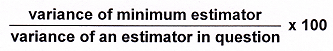
16. EVOP: Stands for evolutionary operation, a term that describes the way sequential experimental designs can be made to adapt to
    system behavior by learning from present results and predicting future treatments for better response. Often, small response improvements may be made via large sample sizes. The experimental risk, however, is quite low because the trials are conducted in the near vicinity of an already satisfactory process.
17. Experiment:  A test is undertaken to make an improvement in a process, or to learn previously unknown information.
18. Experimental error: Variation in response or outcome of virtually identical test conditions. This is also called residual error.
19. First-order: Refers to the power to which a factor appears in a model. If "X₁" represents a factor and "B" is its factor effect, then the model:Y=B₀+B₁X₁+B₂X₂+ε
    is first-order in both X₁ and X₂. First-order models cannot account for curvature or interaction.
20. Fractional: An adjective that means fewer experiments than the full design calls for. The three-factor designs shown below are two-level, half-fractional designs.
21. Full factorial: Describes experimental designs which contain all combinations of all levels of all factors. No possible treatment combinations are omitted. A two-level, three-factor full factorial design is shown below:
22. Inference space: The inference space is the operating range of the factors. It is where the factor's range is used to infer an output to a setting not used in the design. Normally, it is assumed that the settings of the factors within the minimum and maximum
    experimental settings are acceptable levels to use in a prediction equation. For example, if factor A has low and high settings of five and ten units, it is reasonable to make predictions when the factor is at a setting of six. However, predictions at a value of thirteen cannot and should not be attempted because this setting is outside the region that was explored. (For a 2^k design, a check for curvature should be done prior to assuming linearity between the high and low outputs.)
23. Narrow inference: A narrow inference utilizes a small number of test factors and/or factor levels or levels that are close together to minimize the noise in a DOE. One example of a narrow inference is having five machines, but doing a DOE on just one machine to minimize the noise variables of machines and operators.
24. Broad inference: A broad inference utilizes a large number of the test factors and/or factor levels or levels that are far apart, recognizing that noise will be present. An example of a broad inference is performing a DOE on all five machines. There will be more noise, but the results more fully address the entire process.
25. Input factor: An independent variable that may affect a (dependent) response variable and is included at different levels in the experiment.
26. Inner array: In Taguchi-style fractional factorial experiments, these are the factors that can be controlled in a process.
27. Interaction: An interaction occurs when the effect of one input factor on the output depends upon the level of another input factor. Interactions can be readily examined with full factorial experiments. Often, interactions are lost with fractional factorial experiments.
28. Level: A given factor or a specific setting of an input factor. Four levels of heat treatment may be 100°F, 120°F, 140°F, and 160°F.
29. Main effect: An estimate of the effect of a factor independent of any other factors.
30. Mixture experiments: Experiments in which the variables are expressed as proportions of the whole and sum to 1.0.
31. Multicollinearity:  This occurs when two or more input factors are expected to independently affect the value of an output factor but are found to be highly correlated. For example, an experiment is being conducted to determine the market value of a house. The input factors are square feet of living space and the number of bedrooms. In this case, the two input factors are highly correlated. Larger residences have more bedrooms.
32. Nested: An experimental design in which all trials are not fully experimenting randomized. There is generally a logical reason for taking this action. For example, in an experiment, technicians might be nested within labs. As long as each technician stays with the same lab, the techs are nested. It is not often that techs travel to different labs just to make the design balanced.
33. Optimization: This involves finding the treatment combinations that give the most desired response. Optimization can be "maximization" (as, for example, in the case of product yield) or "minimization" (in the case of impurities).
34. Orthogonal: A design is orthogonal if the main and interaction effects in a given design can be estimated without confounding the other main effects or interactions. Two columns in a design matrix are orthogonal if the sum of the products of their elements within each row is equal to zero. A full factorial is said to be balanced, or orthogonal because there is an equal number of data points under each level of each factor. When a factorial experiment is balanced, the design is said to be completely orthogonal. The Pearson correlation coefficient of all of the factor and interaction columns will be zero.
35. Outer array: In a Taguchi-style fractional factorial experiment, these are the factors that cannot be controlled in a process.
36. Paired comparison: The basis of a technique for treating data so as to ignore sample-to-sample variability and focus more clearly on variability caused by a specific factor effect. Only the differences in response for each sample are tested because sample-to-sample differences are irrelevant.
37. Parallel experiments: These experiments are done at the same time, not one after another, e.g., agricultural experiments in a big cornfield. Parallel experimentation is the opposite of sequential experimentation.
38. Precision: The closeness of agreement between test results.
39. Qualitative: This refers to descriptors of category and/or order, but not of interval or origin. Different machines, operators, materials, etc. represent qualitative levels or treatments.
40. Quantitative: This refers to descriptors of order and interval (interval scale) and possibly also of origin (ratio scale). As a quantitative factor, "temperature" might describe the interval value 27.32°C. As a quantitative response, "yield" might describe the ratio value 87.42%.
41. Random factor: A random factor is any factor whose settings (such as any speed within an operating range) could be randomly selected, as opposed to a fixed factor whose settings (such as the current and proposed levels) are those of specific interest to the experimenter. Fixed factors are used when an organization wishes to investigate the effects of particular settings or, at most, the inference space enclosed by them. Random factors are used when the organization wishes to draw conclusions about the entire population of levels.
42. Randomization: Randomization is a technique to distribute the effect of unknown noise variables over all the factors. Because some noise factors may change over time, any factors whose settings are not randomized could be confounded with these time-dependent elements. Examples of factors that change over time are tool wear, operator fatigue, process bath concentrations, and changing temperatures throughout the day.
43. Randomized trials: Frees an experiment from the environment and eliminates biases. This technique avoids the undue influences of systematic changes that are known or unknown.
44. Repeated trials: Trials that are conducted to estimate the pure trial-to-trial experimental error so that lack of fit may be judged. Also called replications.
45. Residual error: The difference between the observed and the predicted value (ε) or (E) for that result, based on an empirically determined model. It can be variation in outcomes of virtually identical test conditions.
46. Residual: The difference between experimental responses and predicted model values. A residual is a measure of the error in a model. A prediction equation estimates the output of a process at various levels within the inference space. These predicted values are called fits. The residual is the difference between a fit and an actual experimentally observed data point.
47. Residual Analysis: Residual analysis is the graphical analysis of residuals to determine if a pattern can be detected. If the prediction equation is a good model, the residuals will be independently and normally distributed with a mean of zero and a constant variance. Nonrandom patterns indicate that the underlying assumptions for the use of ANOVA have not been met. It is important to look for nonrandom and/or non-normal patterns in the residuals. These types of patterns can often point to potential solutions. For example, if the residuals have more than one mode, there is most likely a missing factor. If the residuals show trends or patterns vs. the run order, there is a time-linked factor.
48. Resolution:Resolution is the amount and structure of aliasing of factors and interactions in an experimental design. Roman numerals are used to indicate the degree of aliasing, with Resolution III being the most confounded. A full factorial design has no terms that are aliased. The numeral indicates the aliasing pattern. A Resolution III has main effects and two-way interactions confounded (1+2 = III). A Resolution V has one-way and four-way interactions as well as two-way and three-way interactions aliased (1+4 = V = 2+3).
49. Resolution I: An experiment in which tests are conducted, adjusting one factor at a time, hoping for the best. This experiment is not statistically sound
50. Resolution ll: An experiment in which some of the main effects are confounded. This is very undesirable.
51. Resolution III: A fractional factorial design in which no main effects are confounded with each other, but the main effects and two, factor interaction effects are confounded.
52. Resolution IV: A fractional factorial design in which the main effects and two-factor interaction effects are not confounded, but the two-factor effects may be confounded with each other.
53. Resolution V: A fractional factorial design in which no confounding of main effects and two-factor interactions occur. However, two-factor interactions may be confounded with three-factor and higher interactions.
54. Resolution Vl: Also called Resolution V+. This is at least a full factorial experiment with no confounding. It can also mean two blocks of 16 runs.
55. Resolution Vll: Can refer to eight blocks of 8 runs.
56. Response surface methodology (RSM): The graph of a system response plotted against one or more system factors. Response surface methodology employs experimental design to discover the "shape" of the response surface and then uses geometric concepts to take advantage of the relationships discovered.
57. Response variable: The variable that shows the observed results of an experimental treatment. Also known as the output or dependent variable.
58. Robust design: A term associated with' the application of Taguchi experimentation in which a response variable is considered robust or immune to input variables that may be difficult or impossible to control.
59. Screening: A technique to discover the most (probable) important factors experiment in an experimental system. Most screening experiments employ two-level designs. A word of caution about the results of screening experiments, if a factor is not highly significant, it does not necessarily mean that it is insignificant.
60. Second-order: Refers to the power to which one or more factors appear in a model. If "X1" represents a factor and "B," is its factor effect, then the model: Y= Bo + B1X1 + B11(X1 * X1)+B2X2+ɛ is second-order in X1 but not in X2. Second-order models can account for curvature and interaction. B12(X1 * X1)  is another second-order example, representing an interaction between X1 and X2.
61. Sequential experiments: Experiments are done one after another, not at the same time.  This is often required by the type of experimental design being used. Sequential experimentation is the opposite of parallel experimentation.
62. Simplex: A geometric figure that has a number of vertexes (corners) equal to one more than the number of dimensions in the factor space.
63. Simplex design: A spatial design used to determine the most desirable variable combination (proportions) in a mixture.
64.  The sparsity of effects principle states that processes are usually driven by main effects and low-order interactions.
65. Test coverage: The percentage of all possible combinations of input factors in an experimental test.
66. Treatments: In an experiment, the various factor levels describe how an experiment is to be carried out. A pH level of 3 and a temperature level of 37° Celsius describe an experimental treatment.

Experimental Objectives

Choosing an experimental design depends on the objectives of the experiment and the number of factors to be investigated. Some experimental design objectives are:

1. Comparative objective: If several factors are under investigation, but the primary goal of the experiment is to make a conclusion about whether a factor, in spite of the existence of the other factors, is "significant," then the experimenter has a comparative problem and needs a comparative design solution.
2. Screening objective: The primary purpose of this experiment is to select or screen out the few important main effects from the many lesser important ones. These screening designs are also termed main effects or fractional factorial designs.
3. Response surface (method) objective: This experiment is designed to let an experimenter estimate interaction (and quadratic) effects and, therefore, give an idea of the (local) shape of the response surface under investigation. For this reason, they have termed response surface method (RSM) designs. RSM designs are used to:
   • Find improved or optimal process settings
   • Troubleshoot process problems and weak points
   • Make a product or process more robust against external influences
4. Optimizing responses when factors are proportions of a mixture objective: If an experimenter has factors that are proportions of a mixture and wants to know the "best" proportions of the factors to maximize (or minimize) a response, then a mixture design is required.
5. Optimal fitting of a regression model objective: If an experimenter wants to model response as a mathematical function (either known or empirical) of a few continuous factors, to obtain "good" model parameter estimates, then a regression design is necessary.

Important practical considerations in planning and running experiments are:

• Check the performance of gauges/measurement devices first
•  Keep the experiment as simple as possible
• Check that all planned runs are feasible
•  Watch out for process drifts and shifts during the run
• Avoid unplanned changes (e.g. switching operators at half time)
•  Allow some time (and back-up material) for unexpected events
• Obtain buy-in from all parties involved
• Maintain effective ownership of each step in the experimental plan
• Preserve all the raw data – do not keep only summary averages!
• Record everything that happens
• Reset equipment to its original state after the experiment

Select and Scale the Process Variables

Process variables include both inputs and outputs, I. e. factors and responses. The selection of these variables is best done as a team effort. The team should:

• Include all important factors (based on engineering and operator judgments)
•  Be bold, but not foolish, in choosing the low and high factor levels
• Avoid factor settings for impractical or impossible combinations
• Include all relevant responses
• Avoid using responses that combine two or more process measurements

When choosing the range of settings for input factors, it is wise to avoid extreme values. In some cases, extreme values will give runs that are not feasible; in other cases, extreme ranges might move the response surface into some erratic region. The most popular experimental designs are called two-level designs. Two-level designs are simple and economical and give most of the information required to go to a multi-level response surface experiment if one is needed. However, two-level designs are something of a misnomer. It is often desirable to include some center points (for quantitative factors) during the experiment (center points are located in the middle of the design "box."). The choice of a design depends on the number of resources available and the degree of control over making wrong decisions (Type I and Type II hypotheses errors). It is a good idea to choose a design that requires somewhat fewer runs than the budget permits so that additional runs can be added to check for curvature and to
correct any experimental mishaps.

DOE Checklist

Every experimental investigation will differ in detail, but the following checklist will be helpful for many investigations.

•  Define the objective of the experiment.
• The principle experimenter should learn as many facts about the process as possible prior to brainstorming.
• Brainstorm a list of the key independent and dependent variables with people knowledgeable of the process and determine if these factors can be controlled or measured.
• Run "dabbling experiments" where necessary to debug equipment or determine measurement capability. Develop experimental skills and get some preliminary results.
• Assign levels to each independent variable in the light of all available knowledge.
• Select a standard DOE plan or develop one by consultation. It pays to have one person outline the DOE and another review it critically.
• Run the experiments in random order and analyze results periodically.
• Draw conclusions. Verify by replicating experiments, if necessary, and proceed to follow-up with further experimentation if an improvement trend is indicated in one or more of the factors.

It is often a mistake to believe that "one big experiment will give the answer." A more useful approach is to recognize that while one experiment might give a useful result, it is more common to perform two, three, or more experiments before a complete answer is attained. An iterative approach is usually the most economical. Putting all one's eggs in one basket is not advisable. It is logical to move through stages of experimentation, each stage supplying a different kind of answer.

Experimental Assumptions

In all experimentation, one makes assumptions. Some of the engineering and mathematical assumptions an experimenter can make include:

• Are the measurement systems capable of all responses?
  It is not a good idea to find, after finishing an experiment, that the measurement devices are incapable. This should be confirmed before embarking on the experiment itself. In addition, it is advisable, especially if the experiment lasts over a protracted period, that a check is made on all measurement devices from the start to the conclusion of the experiment. Strange experimental outcomes can often be traced to 'hiccups' in the metrology system.
• Is the process stable?

  Experimental runs should have control runs that are done at the "standard" process setpoints, or at least at some identifiable operating conditions. The experiment should start and end with such runs. A plot of the outcomes of these control runs will indicate if the underlying process itself drifted or shifted during the experiment. It is desirable to experiment on a stable process. However, if this cannot be achieved, then the process instability must be accounted for in the analysis of the experiment.

• Are the residuals (the difference between the model predictions and the actual observations) well behaved?
  Residuals are estimates of experimental error obtained by subtracting the observed response from the predicted response. The predicted response is calculated from the chosen model after all the unknown model parameters have been estimated from the experimental data. Residuals can be thought of as elements of variation unexplained by the fitted model. Since this is a form of error, the same general assumptions apply to the group of residuals that one typically uses for errors in general: one expects them to be normally and independently distributed with a mean of 0 and some constant variance. These are the assumptions behind ANOVA and classical regression analysis. This means that an analyst should expect a regression model to err in predicting response in a random fashion; the model should predict values higher and lower than actual, with equal probability. In addition, the level of the error should be independent of when the observation occurred in the study, or the size of the observation being predicted, or even the factor settings involved in making the prediction. The overall pattern of the residuals should be similar to the bell-shaped pattern observed when plotting a histogram of normally distributed data. Graphical methods are used to examine residuals. Departures from assumptions usually mean that the residuals contain a structure that is not accounted for in the model. Identifying that structure, and adding a term representing it to the original model, leads to a better model. Any graph suitable for displaying the distribution of a set of data is suitable for judging the normality of the distribution of a group of residuals. The three most common types are histograms, normal probability plots, and dot plots. Shown below are examples of dot plot results.

Steps to perform a DOE:

In General

1. Document the initial information.
2.  Verify the measurement systems.
3. Determine if baseline conditions are to be included in the experiment. (This is usually desirable.)
4. Make sure clear responsibilities are assigned for proper data collection.
5. Always perform a pilot run to verify and improve data collection procedures.
6. Watch for and record any extraneous sources of variation.
7.  Analyze data promptly and thoroughly.
8. Always run one or more verification runs to confirm results (i.e., go from a narrow to broad inference).

Setting up a DOE

1. State the practical problem.
   For example, a practical problem may be "Improve yield by investigating factor A and factor B. Use an α of 0.05."
2. State the factors and levels of interest.
   For example, factors and levels of interest could be defined as, "Set coded values for factors A and B at -1 and +1."
3. Select the appropriate design and sample size based on the effect to be detected.
4. Create an experimental data sheet with the factors in their respective columns. Randomize the experimental runs in the datasheet. Conduct the experiment and record the results.
5. Construct an Analysis of Variance (ANOVA) table for the full model.
6. Review the ANOVA table and eliminate effects with p-values above α. Remove these one at a time, starting with the highest order interactions.
7.  Analyze the residual plots to ensure that the model fits.
8.  Investigate the significant interactions (p-value < α). Assess the significance of the highest order interactions first. (For two-way interactions, an interactions plot may be used to efficiently determine optimum settings. For graphical analysis to determine settings for three-way interactions, it is necessary to evaluate two or more interaction plots simultaneously.). Once the highest order interactions are interpreted, analyze the next set of lower-order interactions.
9. Investigate the significant main effects (p-value < α).
   (Note: If the level of the main effect has already been set as a result of a significant interaction, this step is not needed.). The use of the main effects plots is an efficient way to identify these values. Main effects that are part of statistically valid interactions must be kept in the model, regardless of whether or not they are statistically valid themselves. Care must be taken because, due to
   interactions, the settings chosen from the main effects plot may sometimes lead to a sub-optimized solution. If there is a significant interaction, use an interaction plot, as shown in the following chart.
10. State the mathematical model obtained.
    For a 2^k design, the coefficients for each factor and interaction are one-half of their respective effects. Therefore, the difference in the mean of the response from the low setting to the high setting is twice the size of the coefficients.
    Commonly available software programs will provide these coefficients as well as the grand mean. The prediction equation is stated, for two factors,:
    y = grand mean + β₁X₁ + β₂X₂ + β₃(X₁ x X₂)
11.  Calculate the percent contribution of each factor and each interaction relative to the total "sum of the squares." This is also called epsilon squared. It is calculated by dividing the sum of the squares for each factor by the total sum of the squares and is a rough evaluation of "practical" significance.
12. Translate the mathematical model into process terms and formulate conclusions and recommendations.
13. Replicate optimum conditions and verify that results are in the predicted range. Plan the next experiment or institutionalize the change.

Example:

An organization decided that it wanted to improve yield by investigating the pressure and temperature in one of its processes. Coded values for pressure and temperature were set at -1 and +1. The design and sample size chosen involved two replications of a 22 design for a total of eight runs. The experiment was conducted and the results were recorded as shown.

The Analysis of Variance (ANOVA) table for the full model was then constructed:

The ANOVA table was reviewed to eliminate the effects with a p-value above α. Because both main effects and the interaction were below the chosen α of 0.05, all three were included in the final model. The residual plots were analyzed in three ways, to ensure that the model fit:

1. The residuals were plotted against the order of the data using an Individuals Chart and Run Chart to check that they were randomly distributed about zero.
2. A normal probability plot was run on the residuals.
3. A plot of the residuals vs. the fitted or predicted values was run to check that the variances were equal (i.e., the residuals were independent of the fitted values).

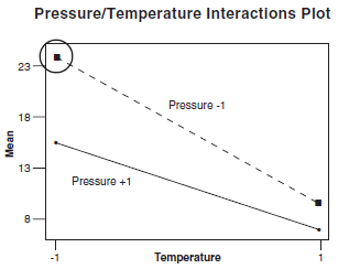
Creating an interactions plot for pressure and temperature showed that the optimum setting to maximize yield was to set both temperature and pressure at -1.

The chosen mathematical model involved the prediction equation:

 y = grand mean + β₁X₁ + β₂X₂ + β₃(X₁ x X₂).

Substituting a grand mean of 14.00 and coefficients of -2.75 for pressure, -5.75 for temperature, and 1.50 for (P x T) into the equation, we get:
y = 14.00 – 2.75(Pressure) – 5.75(Temperature) + 1.5(P x T)
Using the optimum settings of pressure = -1  and
temperature = -1 that were identified earlier forces the setting for the interaction (P x T) to be (-1) x (-1) = +1.

Substituting these values into the prediction equation, we get:
y = 14.00 – 2.75(-1) – 5.75(-1) + 1.5(+1) = 24.00
This equation tells us that, to increase yield, the pressure and temperature must be lowered. The results should be verified via confirmation runs and experiments at even lower settings of temperature and pressure should also be considered.

Selecting Factor setting:

• Process knowledge: Understand that standard operating conditions in the process could limit the range for the factors of interest. Optimum settings may be outside this range. For this reason, choose bold settings, while never forgetting safety.
•  Risk: Always consider those bold settings that could possibly endanger equipment or individuals and must be evaluated for such risk. Avoid settings that have the potential for harm.
• Cost: Cost is always a consideration. Time, materials, and/or resource constraints may also impact the design.
• Linearity: If there is a suspected nonlinear effect, budget for runs to explore for curvature and also make sure the inference space is large enough to detect the nonlinear effect.

Notation:

The general notation to designate a fractional factorial design is:

Where:
• k is the number of factors to be investigated.
• p designates the fraction of the design.
• 2^k-p is the number of runs. For example, a 2⁵ design requires thirty-two runs, a 2^5-1 (or 2⁴) design requires sixteen runs (a half-fractional design), and a 2^5-2 (or 2³) design requires eight runs (a quarter-fractional design).
• R is the resolution.

Coding:

Coding is the representation of the settings picked in a standardized format. Coding allows for a clear comparison of the effects of the chosen factors. The design matrix for 2k factorials is usually shown in standard order. The Yates standard order has the first-factor alternate low settings, then high settings, throughout the runs. The second factor in the design alternates two runs at the low setting, followed by two runs at the high setting.
The low level of a factor is designated with a "-" or -1  and the high level is designated with a "+" or 1.

Coded values can be analyzed using the ANOVA method and yield a y = f (x) prediction equation. The prediction equation will be different for coded vs. uncoded units. However, the output range will be the same. Even though the actual factor settings in an example might be temperature 160° and 180° C, 20% and 40% concentration, and catalysts A and B, all the settings could be analyzed using -1 and +1 settings without losing any validity.

Fractional vs. Full DOEs

There are advantages and disadvantages for all DOEs. The DOE chosen for a particular situation will depend on the conditions involved.
Advantages of full factorial DOEs:

• All possible combinations can be covered.
• Analysis is straightforward, as there is no aliasing.

Disadvantages of full factorial DOEs:
The cost of the experiment increases as the number of factors increases. For instance, in a two-factor two-level experiment (2²), four runs are needed to cover the effect of A, B, AB, and the grand mean. In a five-factor two-level experiment (2⁵), thirty-two runs are required to do a full factorial. Many of these runs are used to evaluate higher-order interactions that the experimenter may not be interested in. In a 23 experiment, there are five one-way effects (A, B, C, D, E), ten two-ways, ten three-ways, five four-ways, and one five-way effect. The 2²experiment has 75% of its runs spent learning about the likely one-way and two-way effects, while the 2⁵design only spends less than 50% of its runs examining these one-way and two-way effects.
Advantages of fractional factorial DOEs:

• Less money and effort is spent for the same amount of data.
• It takes less time to do fewer experiments.
• If data analysis indicates, runs can be added to eliminate confounding.

Disadvantages of fractional factorial DOEs:

• Analysis of higher order interactions could be complex.
• Confounding could mask factor and interaction effects.

Setting up a fractional factorial DOE

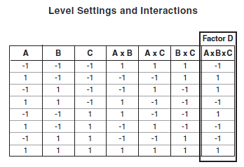
The effect of confounding should be minimized when setting up a fractional factorial. The Yates standard order will show the level settings of each factor and a coded value for all the interactions. For example, when A is high (+1) and B is low (-1), the interaction factor AB is (+1 x -1 = -1). A column for each interaction can thus be constructed as shown here:

Running a full factorial experiment with one more factor (D) would require a doubling of the number of runs. If factor D settings are substituted for a likely insignificant effect, that expense can be saved. The highest interaction is the least likely candidate to have a significant effect. In this case, replacing the A x B x C interaction with factor D allows the experimenter to say ABC was aliased or confounded with D. The three-level interaction still exists but will be confounded with the factor D. All credit for any output change will be attributed to factor D. This is a direct application of the sparsity of effects principle. In fact, there is more aliasing than just D and ABC. Aliasing two-way and three-way effects can also be accomplished and can be computed in two ways:

1.  By multiplying any two columns together (such as column A and column D), each of the values in the new column (AD) will be either -1 or +1. If the resulting column matches any other (in this case, it will match column BC), those two effects can be said to be confounded.
2.  The Identity value (I) can be discovered and multiplied to get the aliased values. For example, in this case, because D=ABC (also called the design generator), the Identity value is ABCD. Multiplying this Identity value by a factor will calculate its aliases. Multiplying ABCD and D will equal ABCDD. Because any column multiplied by itself will create a column of 1's (multiplication identity), the D2 term drops out, leaving ABC and reaffirming that D=ABC.

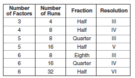
Adding an additional factor to a full factorial without adding any additional runs will create a half fractional design. (The design has half the runs needed for a full factorial. If a design has one-quarter the runs needed for full factorial analysis, it is a quarter fractional design, etc.) The key to selecting the type of run and number of factors is to understand what the resolution of the design is, for any given number of factors and available runs. The experimenter  must decide how much confounding he or she is willing to accept. A partial list of fractional designs is included below.

Interaction Case Study

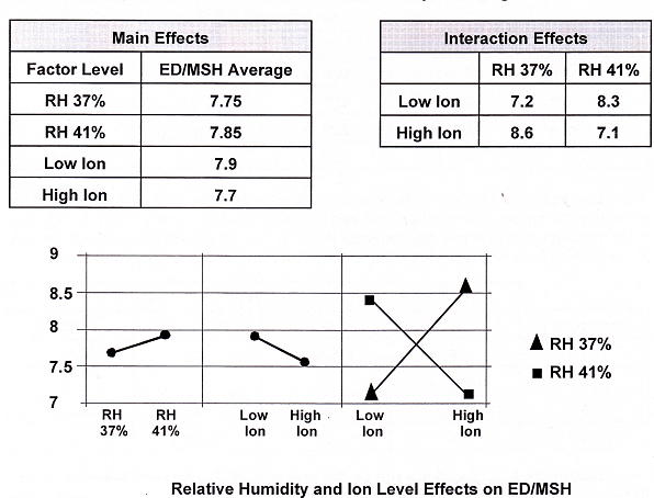
A simple 2 x 2 factorial experiment (with replication) was conducted in the textile industry. The response variable was ED/MSH (ends down/thousand spindle hours.). The independent factors were RH (relative humidity) and ion level (the environmental level of negative ions). Both of these factors were controllable. A low ED/MSH is desirable since fewer thread breaks means higher productivity. An ANOVA showed the main effects were not significant but the interaction effects were highly significant. Consider the data table and plots in Figure below:
The above interaction plot demonstrates that if the goal is to reduce breaks, an economic choice could be made between low ion/low RH and high ion/high RH.

Randomized Block Plans

In comparing, a number of factor treatments, it is desirable that all other conditions be kept as nearly constant as possible. The required number of tests may be too large to be carried out under similar conditions. In such cases, one may be able to divide the experiment into blocks, or planned homogeneous groups. When each group in the experiment contains exactly one measurement of every treatment, the experimental plan is called a randomized block plan. A randomized block design for air permeability response is shown below: An experimental scheme may take several days to complete. If one expects some biasing differences among days, one might plan to measure each item on each day or to conduct one test per day on each item. A day would then represent a block. A randomized incomplete block (tension response) design is shown below: Only treatments A, C, and D are run on the first day. B, C, and D on the second, etc. In the whole experiment, note that each pair of treatments, such as BC, occur twice together. The order in which the three treatments are run on a given day follows a randomized sequence. Blocking factors are commonly environmental phenomena outside of the control of the experimenter.

Latin Square Designs

A Latin square design is called a ope-factor design because it attempts to measure the effects of a single key input factor on an output factor. The experiment further attempts to block (or average) the effects of two or more nuisance factors. Such designs were originally applied in agriculture when the two sources of non- homogeneity (nuisance factors) were the two directions on the field. The square was literally a plot of ground. In Latin square designs, a third variable, the experimental treatment, is then applied to the source variables in a balanced fashion. The Latin square plan is restricted by two conditions:

1.  The number of rows, columns, and treatments must be the same.
2. There should be no expected interactions between row and column factors, since these cannot be measured. If there are, the sensitivity of the experiment is reduced.

A Latin square design is essentially a fractional factorial experiment which requires less experimentation to determine the main treatment results.

Consider the following 5 x 5 Latin square design:In the above design, five drivers and five carburetors were used to evaluate gas mileage from five cars (A, B, C, D, and E). Note that only twenty-five of the potential 125 combinations are tested. Thus, the resultant experiment is a one-fifth fractional factorial. Similar 3 x 3, 4 x 4, and 6 x 6 designs may be utilized. In some situations, what is thought to be a nuisance factor can end up being very important.

Graeco-Latin Designs

Graeco-Latin square designs are sometimes useful to eliminate more than two sources of variability in an experiment. A Graeco-Latin design is an extension of the Latin square design, but one extra blocking variable is added for a total of three blocking variables. Consider the following 4 X 4 Graeco-Latin design: The output (response) variable could be gas mileage for the 4 cars (A, B, C, D).

Hyper-Graeco-Latin Designs

A hyper-Graeco-Latin square design permits the study of treatments with more than three blocking variables. Consider the following 4 x 4 hyper-Graeco-Latin design:

The output (response) variable could be gas mileage for the 4 cars (A, B, C, D).

Two-Level Fractional Factorial Example

The basic steps for a two-level fractional factorial design will be examined via the following hypothetical example. The following seven-step procedure will be followed:

1. Select a process
2. Identify the output factors of concern
3. Identify the input factors and levels to be investigated
4. Select a design (from a catalogue, Taguchi, self created, etc.)
5. Conduct the experiment under the predetermined conditions
6. Collect the data (relative to the identified outputs)
7. Analyze the data and draw conclusions

Step 1: Select a process
We want to investigate UPSC(Union Public Service Commission) Prelims exam success using students of comparable educational levels.
Step 2: Identify the output factors
Student performance will be based on two results (output factors):
(1) Did they pass the test?
(2) What grade score did they receive?
Step 3: Establish the input factors and levels to be investigated
We want to study the effect of seven variables at two-level that may affect student performance. (7 factors at 2-levels)

Input factor	Level 1(-)	Level 2(+)
UPSC coaching	NO	Yes
Study time	Morning	Afternoon
Problem worked	200	800
Primary Reference	Book A	Book B
Method of study	Sequential	Random
Work experience	0 years	4 years +
Duration of study	50 hours	120 hours

Note: The above inputs are both variable (quantitative) and attribute (qualitative).
Step 4: Select a design
A screening plan is selected from a design catalogue. Only eight (8) tests are needed to evaluate the main effects of all 7 factors at 2-levels. The design is:

Input factors
TESTS	A	B	C	D	E	F	G
#1	–	–	–	–	–	–	–
#2	–	–	–	+	+	+	+
#3	–	+	+	–	–	+	+
#4	–	+	+	+	+	–	–
#5	+	–	+	–	+	–	+
#6	+	–	+	+	–	+	–
#7	+	+	–	–	+	+	–
#8	+	+	–	+	–	–	+

One test example:

Test #3 means:

• A (-) = No UPSC coaching
• B (+) = Study in afternoon
• C (+) = Work 800 problems
• D (-) = Use reference book A
• E (-) = Use sequential study method
• F (+) = Have 4 years + of work experience
• G (+) = Study 120 hours for the test

Step 5: Conduct the experiment
Step 6: Collect the data

Step 7: Analyze the data and draw conclusions
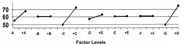
The pass/fail pattern of (+)s and (-)s does not track with any single input factor. It visually appears that there is some correlation with factors C & G

(+) means level 2 has a positive effect. (-) means level 2 has a negative effect. 0 means level 2 has no effect.

• Factor A, taking coaching , will improve the exam results by 13 points
• Factor B, study time of day, has no effect on exam results
• Factor C, problems worked, will improve the exam results by 20 points
• Factor D, primary reference, will improve the exam results by 5 points
• Factor E, method of study, has no effect on exam results
• Factor F, work experience, has no effect on exam results
• Factor G, duration of study, will improve the exam results by 23 points

To calculate the optimum student performance:
1. Sum the arithmetic value of the significant differences (Δ) and divide the total by two. Call this value the improvement. Note that the absolute value is divided by 2 because the experiment is conducted in the middle of the high and low levels and only one—half the difference (Δ) can be achieved.

Improvement = 61 + 2 = 30.5. There were no significant negative effects (-) in this experiment. If there were, they would have been included (added) in determining the total effect. In this particular DOE format, the sign indicates direction only.
2. Average the test scores obtained in tests 1 through 8.
Average = 61.5
3. Add the improvement to the average to predict the optimum performance. .
Optimum = Average + Improvement
= 61.5 + 30.5
= 92
The optimum performance would be obtained by running the following trial: The above trial was one of the 120 tests not performed out of 128 possible choices. Obviously, the predicted student scores can be confirmed by additional experimentation.

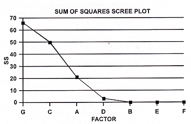
One can further examine the significance of the design results using the sum of squares and a scree plot. A scree plot is so named because it looks like the rubble or rocky debris lying on a slope or at the base of a cliff. The scree plot indicates that factors D, B, E, and F are noise. The SS (sum of squares) for the error term is 3.1 (3.1 + 0 + 0 + 0)
MSE (mean square error) = T =3.1/4= 0.775
The maximum F ratio for factor G Is: 61.5/0.775= 85.29
The critical maximum F value from the following F Table for k – 1 = 7, p = 4 and α = 0.05 is 73. Thus, factor G is important at the 95% confidence level.
The maximum F table accommodates screening designs for runs of 8, 12, 16, 20, and 24. p is the number of noise factors averaged to derive the MSE, and k is the number of runs.
The maximum F ratio for factor C is 50/0.775 = 65.42
The critical maximum F value for k – 1 = 7, p = 4 and d = 0.10 is 49. Thus, factor C is important at the 90% confidence level.
The maximum F ratio for factor A  is 21.1/0.775= 27.22
The critical maximum F values for both alpha values are larger than 27.22. Therefore, factor A is not considered important (at these alpha levels).

A Full Factorial Example

Suppose that pressure, temperature, and concentration are three suspected key variables affecting the yield of a chemical process that is currently running at 64%. An experimenter may wish to fix these variables at two-levels (high and low) to see how they influence yield. In order to find out the effect of all three factors and their interactions, a total of 2 x 2 x 2 = 23 = 8 experiments must be conducted. This is called a full factorial experiment. The low and high levels of input factors are noted below by (-) and (+).
Temperature:    (-) = 120°C        (+) = 150°C
Pressure:              (-) = 10 psi         (+) = 14 psi
Concentration: (-) = 10N             (+) = 12N
To find the effect of temperature, sum the yield values when the temperature is high and subtract the sum of yields when the temperature is low, dividing the results by four.

When the temperature is set at a high level rather than at a low level, one gains 23.5% yield. All of this yield improvement can be attributable to temperature alone since, during the four high temperature experiments, the other two variables were twice low and twice high.

The effect of changing the pressure from a low level to a high level is a loss of 6% yield. Higher concentration levels result in a relatively minor 2% improvement in yield. The interaction effects between the factors can be checked by using the T, P, and C columns to generate the interaction columns by the multiplication of signs: Note, a formal analysis of the above data (developing a scree plot and MSE term) would indicate that only the temperature effect is significant.

 Following the same principles used for the main effects, :* interaction means the change in yield when the pressure and temperature values are both low or both high, as opposed to when one is high and the other is low. The T x P interaction shows a marginal gain in yield when the temperature and pressure are both at the same level.

In this example, the interactions have either zero or minimal negative yield effects.  If the interactions are significant compared to the main effects, they must be considered before choosing the final level combinations. The best combination of factors here is a high temperature, low pressure, and high concentration (even though the true concentration contribution is probably minimal).

Comparison to a Fractional Factorial Design

In some situations, an experimenter can derive the same conclusions by conducting fewer experiments. Suppose the experiments cost Rs 1,00,000 each, one might then decide to conduct a one-half fractional factorial experiment.
Assume the following balanced design is chosen. Since a fractional factorial experiment is being conducted, only the main effects of factors can be determined. Please note that experiments 1, 4, 6, and 7 would have been equally valid. The results are not exactly identical to what was obtained by conducting eight experiments previously. But, the same relative conclusions as to the effects of temperature, pressure, and concentration on the final yield can be drawn. The average yield is 63.25%. If the temperature is high, an 11.75% increase is expected, plus 3.25% for low pressure, plus 1.25% for high concentration equals an anticipated maximum yield of 79.5% even though this experiment was not conducted. This yield is in line with the actual results from experiment number 6 from the full factorial.

MINITAB Results

Most people don't analyze experimental results using manual techniques. The following is a synopsis of the effects of temperature, pressure, and concentration on yield results using MINITAB. This analysis represents the very same data for the previously presented examples.
The F values and corresponding p-values indicate that temperature and pressure are 0 significant to greater than 99% certainty. Concentration might also be important but, more replications would be necessary to see if the 93% certainty could be improved to something greater than 95%.
The regression equation will yield results similar to those for the previous manual calculations. Again, the p-values for temperature and pressure reflect high degrees of certainty.
Using either the manual or MINITAB recaps, would the experimenter stop at this point? Might a follow-up experiment, perhaps at three levels looking at higher temperatures and lower pressures, pay off? After all, the yield has improved by 16% since experimentation started.

DOE Variations

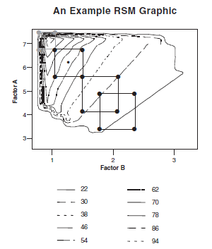
Response Surface Method

The Response Surface Method (RSM) is a technique that enables the experimenter to find the optimum condition for a response (y) given two or more significant factors (x's). For the case of two factors, the basic strategy is to consider the graphical representation of the yield as a function of the two significant factors. The RSM graphic is similar to the contours of a topographical map. The higher up the "hill," the better the yield. Data is gathered to enable the contours of the map to be plotted. Once done, the resulting map is used to find the path of steepest ascent to the maximum or steepest descent to the minimum. The ultimate RSM objective is to determine the optimum operating conditions for the system or to determine a region of the factor space in which the operating specifications are satisfied (usually using a second-order model).

RSM terms:

• Response surface: It is the surface represented by the expected value of an output modeled as a function of significant inputs (variable inputs only):
  Expected (y) = f (x₁, x₂, x₃,…x_n)
• The method of steepest ascent or descent is a procedure for moving sequentially along the direction of the maximum increase (steepest ascent) or maximum decrease (steepest descent) of the response variable using the first-order model:
  y (predicted) = β₀ + Σ β_i x_i
• The region of curvature is the region where one or more of the significant inputs will no longer conform to the first-order model. Once in this region of operation, most responses can be modeled using the following fitted second-order model:
  y (predicted) = β₀ + Σ β_i x_i + Σ β_ii x_ix_i +  Σ β_ij x_ix_j
• The central composite design is a common DOE matrix used to establish a valid second-order model.

Steps for Response Surface Method

1. Select the y. Select the associated confirmed x's and boldly select their experimental ranges. These x's should have been confirmed to have a significant effect on the y through prior experimentation.
2. Add center points to the basic 2^k-p design. A center point is a point halfway between the high and low settings of each factor.
3. Conduct the DOE and plot the resulting data on a response surface.
4. Determine the direction of the steepest ascent to an optimum y.
5. Reset the x values to move the DOE in the direction of the optimum y. In general, the next DOE should have x values that overlap those used in the previous experiment.
6. Continue to conduct DOEs, evaluate the results, and step in the direction of the optimal y until a constraint has been encountered or the data shows that the optimum has been reached.

7. Add additional points to the last design to create a central composite design to allow for a second-order evaluation. This will verify if the analysis is at a maximum or minimum condition. If the condition is at an optimum solution, then the process is ended. If the second-order evaluation shows that the condition is not yet at optimum, it will provide direction for the next sequential experiment.

RSM is intended to be a sequence of experiments with an attempt to "dial in to an optimum setting." Whenever an apparent optimum is reached, additional points are added to perform a more rigorous second-order evaluation.

Plackett-Burman Designs:

Plackett-Burman designs are used for screening experiments. Plackett- Burman designs are very economical. The run number is a multiple of four rather than a power of 2. Plackett-Burman geometric designs are two-level designs with 4, 8, 16, 32, 64, and  128 runs and work best as screening designs. Each interaction effect is confounded with exactly one main effect. All other two-level Plackett-Burman designs (12, 20, 24, 28, etc.) are non-geometric designs. In these designs, a two-factor interaction will be partially confounded with each of the other main effects in the study. Thus, the non-geometric designs are essentially "main effect designs," when there is reason to believe that any interactions are of little significance. For example, a Plackett-Burman design in 12 runs may be used to conduct an experiment containing up to 11 factors. With a 20-run design, an experimenter can do a screening experiment for up to 19 factors. As many as 27 factors can be evaluated in a 28-run design.

Plackett-Burman designs are orthogonal designs of Resolution III that are primarily used for screening designs. Each two-way interaction is positively or negatively aliased with the main effect.
Advantages:
• A limited number of runs are needed to evaluate a lot of factors.
• Clever assignment of factors might allow the Black Belt to determine which factor caused the output, despite aliasing.
Disadvantages:
• It assumes the interactions are not strong enough to mask the main effects.
• Aliasing can be complex.

A Design from a Design Catalogue

The preferred DOE approach examines (screens) a large number of factors with highly fractional experiments. Interactions are then explored or additional levels examined once the suspected factors have been reduced. A one-eighth fractional factorial design is shown below. A total of seven factors are examined at two levels. In this design, the main effects are independent of interactions, and six independent, two-factor interactions can be measured. This design is an effective screening experiment. This particular design comes from a design catalog. Often experimenters will obtain a design generated by a statistical software program. Since this is a one-eighth fractional factorial, there are seven other designs that would work equally as well.
Often, a full factorial or three-level fractional factorial trial (giving some interactions) is used in the follow-up experiment.
Note: 0 = low level and 1 = high level.

A Three-Factor, Three-Level Experiment

Often, a three-factor experiment is required after screening a large number of variables. These experiments may be full or fractional factorial. A one-third fractional factorial design is shown below. Generally, the (-) and (+) levels in two-level designs are expressed as O and 1 in most design catalogues. Three-level designs are often represented as O, 1, and 2.

From a design catalogue test plan, the selected fractional factorial experiment looks
EVOP and PLEX designs

Evolutionary operation (EVOP) is a continuous improvement design. Plant experimentation (PLEX) is a sequence of corrective designs meant to obtain rapid improvement. Both designs are typically small full factorial designs with possible entry points. They are designed to be run while maintaining production; therefore, the inference space is typically very small. EVOP (evolutionary operations) emphasizes a conservative experimental strategy for continuous process improvement. Tests are carried out in phase A until a response pattern is established. Then phase B is centered on the best conditions from phase A. This procedure is repeated until the best result is determined. When nearing a peak, the experimenter will then switch to smaller step sizes or will examine different variables. EVOP can entail small incremental changes so that little or no process scrap is generated. Large sample sizes may be required to determine the appropriate direction of improvement. The method can be extended to more than two variables, using simple main effects experiment designs. The experiment naturally tends to change variables in the direction of the expected improvement, and thus, follows an ascent path. In EVOP experimentation there are few considerations to be taken into account since only two or three variables are involved. The formal calculation of the direction of the steepest ascent is not particularly helpful.

Advantages:

• They do not disrupt production and can be used in an administrative situation.
• They force the organization to investigate factor relationships and prove factory physics.

Disadvantages:

• They can be time-consuming. For example, because, in PLEX, levels are generally set conservatively to ensure that production is not degraded, it is sometimes difficult to prove statistical validity with a single design. A first design may be used to simply decide factor levels for a subsequent design.
• They require continuous and significant management support.

Box-Wilson (central composite) design:

A Box-Wilson design is a rotatable design (subject to the number of blocks) that allows for the identification of nonlinear effects. Rotatability is the characteristic that ensures constant prediction variance at all points equidistant from the design center and thus improves the quality of prediction. The design consists of a cube portion made up from the characteristics of 2^k  factorial designs or 2^k-n fractional factorial designs, axial points, and center points.

Advantages:

• It is a highly efficient second-order modeling design for quantitative factors.
• It can be created by adding additional points to a 2^k-pdesign, provided the original design was at least Resolution V or higher.

Disadvantages:

• It does not work with qualitative factors.
•  Axial points may exceed the settings of the simple model and may be outside the ability of the process to produce.

Box-Behnken design:

A Box-Behnken design looks like a basic factorial design with a center point, except that the corner points are missing and replaced with points on the edges. This type of design is used when the corner
point settings are impossible or impractical because of their combined severity. Running three factors at their high settings could produce a volatile situation.

Advantages:

• It is more efficient than three-level full factorials.
• It is excellent for trials where corner points are not recommended.
• It allows all two-factor interactions to be modeled.
• It can identify interactions and quadratic effects.

Disadvantages:

• Enough trials must be run to estimate all one way and two-way effects (even if only one-way effects are of interest).
• It is hard to modify into other studies.

Subscribe to get access

Read more of this content when you subscribe today.

Back to Home Page

If you need assistance or have any doubt and need to ask any question  contact us at: preteshbiswas@gmail.com. You can also contribute to this discussion and we shall be very happy to publish them in this blog. Your comment and suggestion is also welcome.

Design of Experiments May Be Used With Discerete

Source: https://isoconsultantkuwait.com/2020/11/27/design-of-experiments/

Share this post